AI is very popular right now, and making an AI model is much easier than many expect. For this example, we will make a small fraud detector using XGBoost and Scikit-learn. You can view the Jupyter notebook and other documents I'll be using in this Github repo.
Who This Blog Post is Aimed For
This blog post is aimed for those with at least a bit of experience with Python and coding in general. It would be helpful with some experience with ML.
Before We Begin: Small Reality Check
What you're making is a beginner project. Real fraud detecting is much harder, because
patterns drift over time. The patterns the AI detects in one year may be completely obsolete
in the next few years. A real fraud detector uses something similar to this:
- DDG-DA (Data Distribution Generation for Predictable Concept Drift Adaption)
- Detects changes and adapts accordingly to drift
- TFT (Temporal Fusion Transformer)
- Pattern finder
However, for this tutorial we would only be using a Kaggle data, so our model will not
be accurate. However, it's still great for a learning project.
Prerequisites
We will be using this dataset from Kaggle. We would also need the following Python dependencies. I'm assuming you have
Jupyter notebook installed.
pandas==2.2.2
scikit-learn==1.2.2
matplotlib==3.9.2
seaborn==0.13.2
xgboost==2.1.1
joblib==1.3.2
If you don't know what the dependencies do, that's totally fine. I'll explain it once we use them.
Understanding the Data
Let's take a look at creditcard.csv. I'll quickly explain what the headings mean.
Time
Number of seconds elapsed between this transaction and the first transaction in the dataset
V1-V28
These are values that 'may be result of a (Principal Component Analysis) Dimensionality reduction to protect user identities and sensitive features'. That means that the data is transaction data, just turned into a non-readable form so sensitive information is kept safe. The AI can still use this to detect patterns.
Amount
Transaction amount
Class
1 for fraudulent, 0 for not fraud.
Step 1. Load the data.
import pandas as pd

# Read the CSV
df = pd.read_csv("creditcard.csv")

# Look at first few rows
print(df.head())
print(df['Class'].value_counts(normalize=True))
We are using pandas to read our creditcard.csv, and print
the first few values of the data we're going to use.
Step 2. Look at Class Imbalance
Fraud is rare (thankfully), so this dataset is very imbalanced. Let's take a look.
import seaborn as sns
import matplotlib.pyplot as plt

sns.countplot(x="Class", data=df)
plt.title("Class distribution: Legit (0) vs Fraud (1)")
plt.show()

print(df['Class'].value_counts())
print(df['Class'].value_counts(normalize=True))
The code uses Seaborn to generate the graph, which is show through matplotlib. Seaborn is a very useful tool, as it's very easy to use it to analyse Pandas data, like our df variable.
Your graph should look something like this:
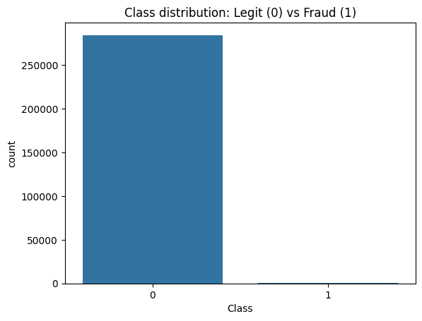
Let's take a look at the graph it made. As you can see, the dataset contains 284315 genuine transactions, and only 492 fraudulent ones. That's a very small amount.
Step 3. Split the Dataset
We need data to both train and test our dataset on. Training without testing is like giving homework to a student and removing the end-of-year exam. For this example, 75% of the data will be used to train, and 25% will be used to test. Fortunately, Scikit-learn has a fantastic function that makes this process a breeze.
from sklearn.model_selection import train_test_split

x_train, x_test, y_train, y_test = train_test_split(
    df.drop('Class', axis=1), df['Class'], test_size=0.25, random_state=42, stratify=df['Class']
)

print("Train shape:", x_train.shape, "Test shape:", x_test.shape)
In machine learning, x_train is the training data’s input features (everything excluding Class header), and y_train is the corresponding target output that the model learns to predict (the Class header).
Step 4. Train the data
from xgboost import XGBClassifier
scale_pos_weight = (y_train == 0).sum() / (y_train == 1).sum()

model = XGBClassifier(
    use_label_encoder=False,
    eval_metric='logloss',
    scale_pos_weight=scale_pos_weight,
    n_estimators=100,
    max_depth=5
)

model.fit(x_train, y_train)
You might be wondering, what does scale_pos_weight do? In Step 2, we saw that a very large majority of the dataset is genuine transactions, while only a small amount is fraud. Our scale_pos_weight basically tells XGBoost that our datasets are imbalanced, and fraudulent data should be 284315 / 492 times more important than non-fraudulent data.
About XGBoost and XGBClassifier?
XGBoost stands for eXtreme Gradient Boosting. It's an ensemble learning method that combines many decision trees (computational trees of wisdom!), and sequentially combines them to make decisions. XGBoost uses many models (trees) working together, and each tree tries to correct the mistakes of the previous ones, so the result is very highly trained model. It's very popular in AI competitions, such as the ones hosted by Kaggle.
What's XGBClassifier? XGBClassifier is a machine learning model from XGBoost. It's designed for classification problems like fraud vs not fraud, scam vs not scam, etc. This fits our use very well.
Step 5. Making some Predictions
Let's use the model we trained to predict some values, and measure the model's precision.
from sklearn.metrics import average_precision_score, classification_report

y_pred = model.predict(x_test)
y_pred_proba = model.predict_proba(x_test)[:, 1]

print("\nClassification Report:")
print(classification_report(y_test, y_pred))

ap = average_precision_score(y_test, y_pred_proba)
print("AUPRC:", ap)
Step 6. Save our Model Locally
Now that we have a trained model, let's download it.
import joblib
joblib.dump(model, 'fraud_detector_model.pkl')
The .pkl extension stands for "pickle", Python's pickle serialisation format.
Loading our Model
To load our model for reuse, we simply do this:
import joblib
loaded_model = joblib.load('fraud_detector_model.pkl')
Analysing the Results
Now let's analyse the model we made. Here are the results you should get:
Classification Report:
              precision    recall  f1-score   support

           0       1.00      1.00      1.00     71079
           1       0.88      0.80      0.84       123

    accuracy                           1.00     71202
   macro avg       0.94      0.90      0.92     71202
weighted avg       1.00      1.00      1.00     71202

AUPRC: 0.8499690863182396
Precision
When the model flags a transaction at fraud, it's correct 88% of the time.
Recall
This model catches 80% of all fraud.
F1 Score
F1 is a way of mixing our precision and recall values. This is the equation:
0.84 is a good value, considering this is a simple demonstration.
Accuracy
The value (1) is wrong, because our dataset is very imbalanced. Even a model that guesses everything as 'not fraud' will get it correct almost every time, which is why this value is displayed as 1.
AUPRC
AUPRC stands for Area Under the Precision-Recall Curve. It's a better way of measuring how well our data is doing with classifying fraud and non-fraud data. It's particularly good at describing imbalanced datasets, like our one. 1 shows that our model is perfect, while 0 means our model is horrible. Our model has an AUPRC of 0.85, which is quite good.
Making a Confusion Matrix
Let's generate a confusion matrix to get a visual representation of our model's accuracy.
from sklearn.metrics import confusion_matrix, ConfusionMatrixDisplay

cm = confusion_matrix(y_test, y_pred)
disp = ConfusionMatrixDisplay(confusion_matrix=cm, display_labels=['Not Fraud', 'Fraud'])

disp.plot(cmap='Blues')
plt.title("Confusion Matrix for Fraud Detection")
plt.show()
Your confusion matrix should look like this:
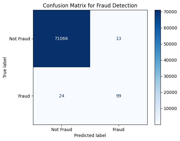
The confusion matrix shows a very dark blue square in the top-left corner, meaning the model correctly identifies almost all non-fraud transactions. The other boxes are much lighter, showing that fraud cases are much fewer and the model doesn’t detect them as accurately.
Conclusion
And there you have it. You have successfully made a machine learning model with XGBoost and Scikit-learn that can detect fraud to a certain degree of precision.
Here are ways to build on to this demo:
- Integrate this into your own programs
- Use advanced ML models or ensemble techniques to increase our model's accuracy.
- Use techniques such as SMOTE or RandomOverSampler
- Play around with the parameters to find the values that maximise the performance.
Thank you for reading. See you in the next one!